Purpose and Scope

This document provides a precise reference specification for the Python class QBitwave, used in the associated manuscripts. It formalizes the mapping from discrete bitstrings to emergent complex amplitudes and describes derived quantities such as Shannon entropy, compressibility, and coherence.

Preliminaries

Let:

• \(b = (b_1,\dots,b_N) \in \{0,1\}^N\) denote a bitstring of length \(N\).

• \(B = \{0,1\}^N\) denote the set of all bitstrings of length \(N\).

• \(n_\text{block}\) denote the block size for bit-to-amplitude conversion (even integer).

• \(\mathbb{C}\) denote the complex numbers.

• \(\|\cdot\|_2\) denote the Euclidean norm.

Forward Mapping: Wavefunction to Bitstring

Given normalized complex amplitudes \(\psi = (\psi_1, \dots, \psi_M) \in \mathbb{C}^M\) and associated phases \(\phi = (\phi_1,\dots,\phi_M)\): \[\begin{aligned} \psi_j &= r_j e^{i \phi_j}, \quad r_j = |\psi_j|, \quad j = 1,\dots,M, \\ b_\text{amp}^j &= \text{binary\_encode}(r_j, k_\text{amp}), \\ b_\text{phase}^j &= \text{binary\_encode}\left(\frac{\phi_j}{2\pi}, k_\text{phase}\right), \end{aligned}\] where \(k_\text{amp}, k_\text{phase}\) are user-selected bits per amplitude/phase. The flattened bitstring is \[b = \bigoplus_{j=1}^M \bigl( b_\text{amp}^j \, || \, b_\text{phase}^j \bigr),\] with \(||\) denoting concatenation.

Reverse Mapping: Bitstring to Wavefunction

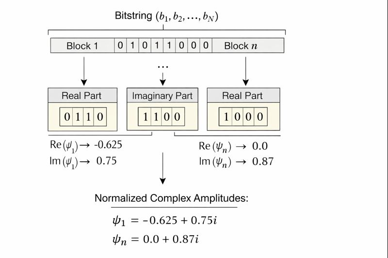
Partition the input bitstring \(b\) into consecutive blocks of size \(n_\text{block}\): \[\begin{aligned} b &= (b_1, \dots, b_N), \quad n_\text{block} \mid N, \\ n_\text{blocks} &= N / n_\text{block}. \end{aligned}\]

Each block is split into two halves (real and imaginary parts): \[\begin{aligned} \text{Re}(\psi_j) &= \text{bits\_to\_signed\_float}\left(b_{(j-1)n_\text{block}+1:j n_\text{block}/2}\right), \\ \text{Im}(\psi_j) &= \text{bits\_to\_signed\_float}\left(b_{j n_\text{block}/2+1:j n_\text{block}}\right), \end{aligned}\] and then normalized: \[\psi = \frac{\psi}{\|\psi\|_2}.\]

Derived Quantities

Amplitude Probabilities

\[p_j = |\psi_j|^2, \quad \sum_{j=1}^M p_j = 1.\]

Shannon Entropy of Wavefunction

\[S_\psi = - \sum_{j=1}^M p_j \log_2 p_j.\]

Bitstring Entropy (Syntactic Entropy)

Let \(p_0, p_1\) be the fractions of zeros and ones in \(b\): \[H_b = -p_0 \log_2 p_0 - p_1 \log_2 p_1.\]

Coherence

The Kullback–Leibler divergence between bit-level and amplitude-level distributions: \[D_\text{KL}(P_b \parallel P_\psi) = \sum_{i=0,1} P_b(i) \log_2 \frac{P_b(i)}{P_\psi(i)},\] where \(P_\psi\) is truncated/aligned to the same length as \(P_b\).

Compressibility

Define the Fourier transform of amplitudes: \[\hat{\psi} = \text{FFT}(\psi),\] and let \(N_\text{sig}\) be the number of Fourier coefficients with magnitude above threshold \(\tau\). Then \[C = 1 - \frac{N_\text{sig}}{M}, \quad C \in [0,1].\]

Randomization / Mutation Operations

Small perturbations of the amplitudes \(\psi \to \psi + \eta\), with \(\eta \sim \mathcal{CN}(0, \sigma^2)\) (complex Gaussian), are normalized to unit norm. Random bit flips on \(b\) trigger automatic recomputation of \(\psi\).

API Summary (Illustrative)

from qbitwave import QBitwave

bw = QBitwave(bitstring)
amps = bw.get_amplitudes()
entropy = bw.entropy()
bit_entropy = bw.bit_entropy()
coherence = bw.coherence()
compress = bw.compressibility()
bw.mutate(level=0.01)
bw.flip(n_flips=5)

Relation to Theory in Main Text

The following properties are essential to the analytical results:

• Normalization of amplitudes

• Mapping from bitstring to complex amplitudes

• Computation of Shannon entropy and compressibility

All other methods (e.g., random flips, mutation) are ancillary and used only in simulation studies.