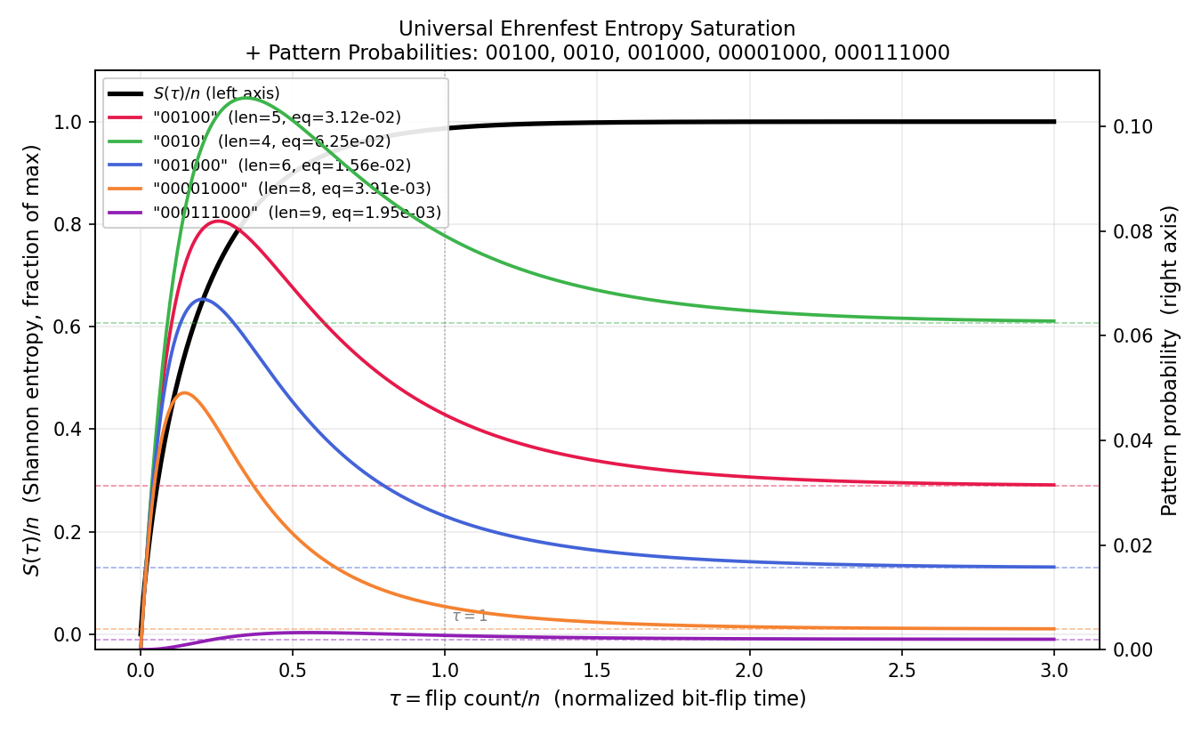
(1 − e−2τ) derived in Section 2, precipitating a freeze-out of
background L0 fabrics. The decoded spatial extent expands, following this closed-form approach to
equilibrium.
(1 − e−2τ) derived in Section 2, precipitating a freeze-out of
background L0 fabrics. The decoded spatial extent expands, following this closed-form approach to
equilibrium.
Starting from the pristine H = 0 boundary state, the following macroscopic phenomena emerge consistently as entropy increases:
Zero entropy yields a structureless state. The all-zero configuration contains no detectable structural matches (NG = 0), mapping naturally under any relational decoding scheme to a single, unextended spatial point. This is the initial state – the singularity.
Spatial expansion. As entropy grows, the density of 1-bits climbs toward 0.5 following the
exact relaxation curve p(τ) = (1 − e−2τ) derived in Section 2, precipitating a freeze-out of
background L0 fabrics. The decoded spatial extent expands, following this closed-form approach to
equilibrium.
Three regimes of structural abundance. For a fixed pattern of length k = a + b (with a ones and b zeros) counted against a bitstring whose global 1-density p(τ) sweeps monotonically from 0 to 1∕2, the expected count is proportional to pa(1 − p)b. This function’s unconstrained maximiser is p∗ = a∕(a + b). Since p(τ) only ever reaches the range [0,1∕2], the observed shape depends entirely on where p∗ falls relative to that range:
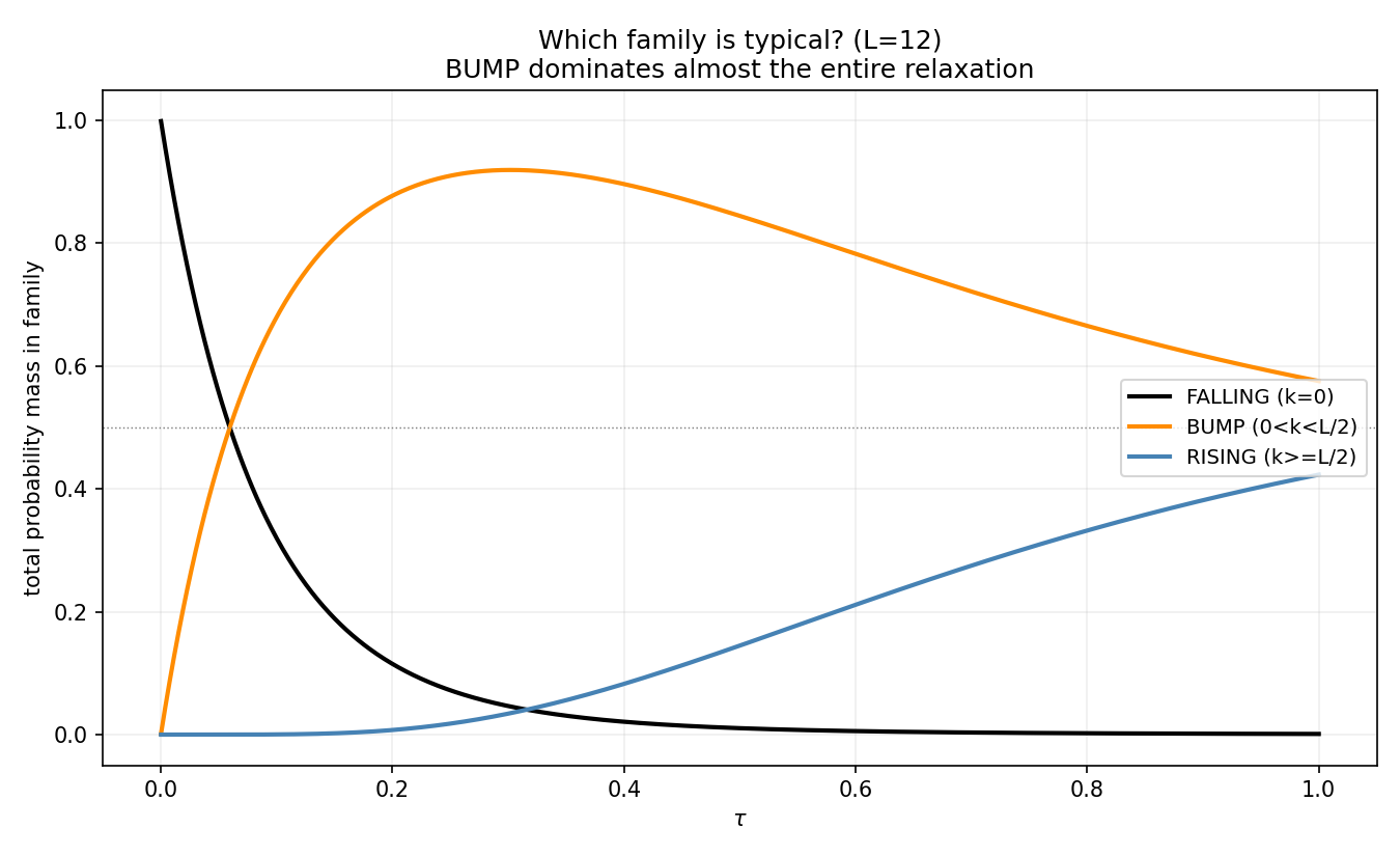
The classification above answers which shape a given composition (a,b) produces. A distinct question is
which class is typical: if a window of fixed length k = a + b is drawn at time τ, which regime does its
observed composition tend to fall into? Answering this requires weighting each composition by the number
of arrangements that share it,  , rather than examining a single representative pattern in
isolation.
, rather than examining a single representative pattern in
isolation.
The number of 1-bits in a length-k window is distributed as Binomial k, p(τ)
 . Since p(τ) ∈ [0,
 ) for
every finite τ, the mean and mode of this distribution lie strictly inside the hump region a < b throughout
the relaxation, approaching the a = b boundary only as τ →∞. Formally, define the composition-weighted
probability mass in each regime:
) for
every finite τ, the mean and mode of this distribution lie strictly inside the hump region a < b throughout
the relaxation, approaching the a = b boundary only as τ →∞. Formally, define the composition-weighted
probability mass in each regime:

with Mhump + Mnon-hump = 1 by construction.
Direct evaluation, with the crossover τc(k) located by root-finding on Mhump(τ) − Mnon-hump(τ) = 0,
shows that Mhump(τ) holds the overwhelming majority of the mass from just above τ = 0 up to τc(k), and
that τc(k) grows with k, with p(τc) → as k →∞:
| k | τc (crossover) | p(τc) |
| 12 | 1.257 | 0.4595 |
| 40 | 1.849 | 0.4876 |
| 100 | 2.304 | 0.4950 |
| 200 | 2.650 | 0.4975 |
| 400 | 2.996 | 0.4988 |
| 1000 | 3.454 | 0.4995 |
 .
.The hump regime is therefore not merely one of three equally weighted possibilities: it is the typical outcome of the relaxation process at any window length, dominating essentially the entire trajectory. The non-hump regimes only attain majority mass in the immediate approach to final equilibrium — a fraction of the trajectory that shrinks as k grows, vanishing entirely in the k →∞ limit except at τ →∞ itself.
This is a fully predictive, closed-form classification: the qualitative shape of any given filter’s abundance curve can be determined in advance from (a,b) alone, without running the simulation.