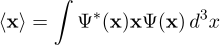
To make any sense out of this, let’s implement it as a software.
Since we want to begin with the material taught in a first QM course, let us start with a minimal single-particle description. This is not QFT yet, but it is a useful stepping stone.
Particles appear quite trivial as classes with only a couple of attributes, plus the wavefunction that contains all the information about the system.
class Particle {
   double mass;          // Rest mass
   double charge;        // Coupling to electromagnetic field
   double spin;          // 0, 0.5, 1.0 etc.
   Wavefunction wavefunction; // Superposition of modes
   Vector3 getExpectedPosition(double time) {
       // Compute center-of-mass from interference pattern
   }
};
The wavefunction is a superposition of modes. Each mode is essentially a complex exponential (plane wave) characterized by wavenumber and phase.
The first approach (momentum primary) aligns well with physics textbooks:
class Mode {
   Vector3 k;       // Wavenumber, p = \hbar k
   complex<double> amplitude; // Complex magnitude & phase
   double phase;    // Initial phase offset
   double frequency() {
     // Natural units: h = c = 1
     return k.squaredNorm() / (2.0 * m); // $\omega = \frac{k^2}{2m}$
   }
};
The wavefunction is then Ψ(x,t) = ∑ ici exp(i(ki ⋅ x − ωit)), or in the continuum limit an integral. A single mode is completely delocalized. As we so intuitively explained it in the previous chapter, localization arises from interference of many modes forming a wave packet.
Wavefunction createWavePacket(Vector3 center, Vector3 width) {
   // Sum many k-modes with Gaussian envelope in momentum space
}
Position is not a fundamental attribute of the Particle. It emerges as the expectation value:
So we have a pretty intuitive design here: a base Particle class with just a couple of attributes, which different kinds of particles inherit from. And as we know from particle physics, some particles are actually made of others. To handle this, we can implement a Group class with a list attribute, letting us group elementary particles together to form composite ones like protons and neutrons.
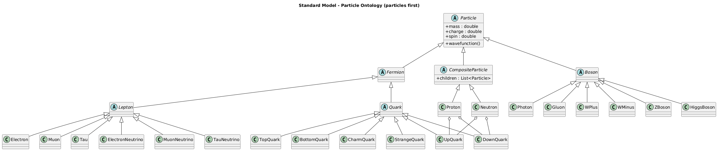
Unfortunately, this intuitive single-particle description already fails for high energies (pair production, variable particle number) and does not incorporate special relativity properly. But we insisted to design the particle class to serve as a pedagogical starting point only.
In order to switch to QFT we must abandon the single-particle picture. According to quantum field theory, the fundamental entities are fields that exist everywhere. Particles are quanta of the fields; localized particles arise as wave packets of those excitations. Unlike a classical field, a quantum field is operator-valued and capable of creating or annihilating particle excitations. To simulate the Standard Model we need multiple fields, one for each fundamental degree of freedom (with appropriate spin and gauge representation).
The true conceptual jump from ordinary quantum mechanics to quantum field theory is not relativity alone. It is the abandonment of fixed particle number.
In introductory QM, one typically studies a wavefunction describing exactly one particle:

or perhaps a fixed number of particles:

The number of particles is assumed from the beginning and never changes. This works remarkably well for low-energy systems such as atoms, molecules, and condensed matter systems.
However, at sufficiently high energies, nature does not respect this restriction. Particles can be created, annihilated, or transformed into entirely different particles:


A fixed-particle Hilbert space is therefore no longer sufficient. We need a framework capable of describing states with arbitrary particle number.
This leads to the idea of second quantization.
Instead of tracking individual particles directly, QFT tracks the occupation of field modes.
For each momentum mode k, we associate an occupation number:

A quantum state is then described by listing how many quanta occupy each mode:

This is called a Fock state.
The vacuum state contains no particles at all:

A single-particle excitation with momentum k is created by applying a creation operator:

Two identical bosons in the same mode:

The operators satisfy algebraic rules encoding quantum statistics.
For bosons:
![[a(k),a†(k ′)] = δ(3)(k − k ′)](ghghnd55x.svg)
For fermions:

The fermionic anticommutation relation automatically produces the Pauli exclusion principle:

Meaning that two identical fermions cannot occupy the same quantum state.
The quantum field itself is no longer an ordinary function. It becomes an operator-valued object:

Roughly speaking, the field operator is built from all creation and annihilation modes:

This expression is enormously important conceptually.
The annihilation operator removes a particle from a momentum mode. The creation operator adds one. The field therefore becomes a machine capable of changing particle number dynamically.
In this sense, particles are no longer fundamental objects. They are excitations generated by the field operators acting on the vacuum.
In ordinary QM, one could imagine the wavefunction as a single object being updated over time.
In QFT, the architecture changes completely.
The system now resembles:
Conceptually, the theory behaves less like a simulation of individual particles and more like a distributed state machine operating on an infinite-dimensional Hilbert space.
The familiar “particle” picture survives only as an approximation valid when localized excitations behave independently.
In the free theory, a quantum field in momentum space is equivalent to a set of harmonic oscillators, one per momentum mode.
class QuantumField {
   const double m;  // Mass of quanta of this field
   // In practice: continuous or discretized over a box
   std::map<Vector3, QuantumOscillator> modes; // or FFT-based grid

   void createParticle(Vector3 k, double amplitude = 1.0) {
       modes[k].n++;          // Apply creation operator
       // In full QFT this acts on the Fock state
   }
};
In QM the Position is an output (an eigenvalue/observable). In QFT, fields are defined over spacetime coordinates, so spacetime labels become part of the field definition itself. A Field is essentially a std::vector or grid where the index is the position x, and the value at that index is the field strength ϕ(x).
The Standard Model uses Minkowski Space. Technically, this is a vacuum solution to the Einstein field equations of General Relativity where the energy-momentum tensor is zero. It describes a flat, four-dimensional manifold where time and space are woven into a single fabric with Lorentzian metric signature of (− + ++) rather than the Euclidean (+ + ++) metric. It is a trivial, hardly worth mentioning, really. We’ll get back to the actual curvature and gravity mess once we get the basic physics engine running without crashing. For now, just assume the “position” is a point on this manifold described by a Four-Vector:

When a new particle is created, we just increment the field counter. However, this is not quite right. A realistic implementation needs creation and annihilation operators a†(k), a(k) satisfying the appropriate commutation (bosons) or anticommutation (fermions) relations, acting on the Fock vacuum |0⟩. No big deal either.
Now that we have Field class, one might expect that the universe could be composed as an array of fields. However, the fields are not all alike, several different field classes are needed (with the correct Lorentz transformation properties).
class Universe {
   // Middleware for mass generation
   HiggsField backgroundField;

   // Fermion sectors (The ’Legacy’ code that was copy-pasted 3 times)
   Generation firstGen {Electron, UpQuark, DownQuark, ElectronNeutrino};
   Generation secondGen {Muon, CharmQuark, StrangeQuark, MuonNeutrino};
   Generation thirdGen {Tau, TopQuark, BottomQuark, TauNeutrino};

   // Gauge Bosons (The ’Communication Protocol’ handlers)
   GluonField strongForce; // SU(3)
   W_Z_Fields weakForce;   // SU(2)
   PhotonField emForce;    // U(1)
};
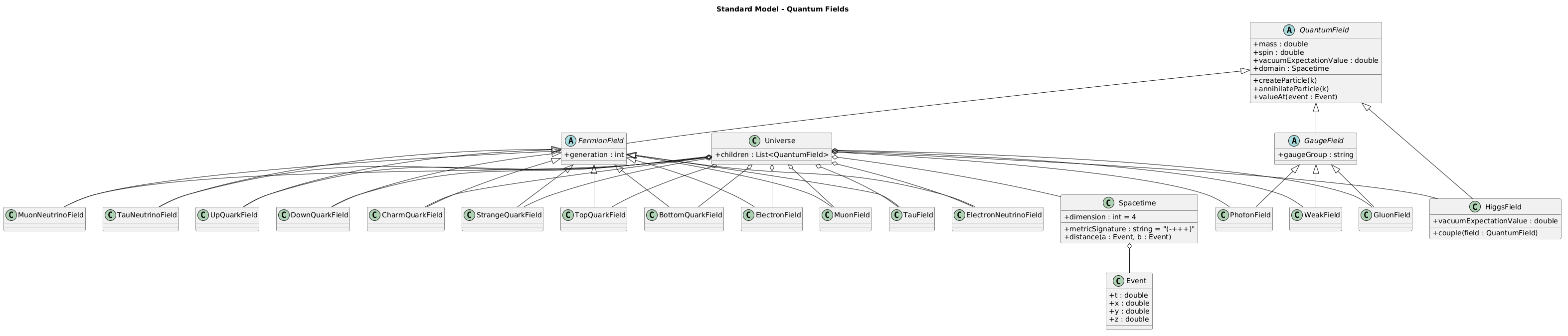
Each field carries its own quantum numbers (representations under the gauge group U(1)Y ×SU(2)L ×SU(3)c). Interactions arise from coupling terms in the Lagrangian (Yukawa, gauge covariant derivatives, etc.), not from manually checking wave overlap.
When a field excitation interacts with a macroscopic detector, the delocalized state becomes entangled with the environment. From the observer’s perspective this appears as a “collapse” to a definite outcome, with probability given by |Ψ(x)|2 (Born rule).
In a full relativistic QFT treatment one must be careful with causality and avoid instantaneous collapse. One can’t have information traveling faster than the speed of light.
The local phase of a field’s wavefunction can change at any point. To maintain physical consistency, one must then introduce a new field to compensate for these local shifts.
| Symmetry Group | Gauge Fields | Physical Bosons |
| U(1)Y | Bμ | mixes into Photon and Z |
| SU(2)L | Wμ1,Wμ2,Wμ3 | W± and part of Z |
| SU(3)c | Gμa | Gluons |
Starting from the familiar single-particle QM class, we have gradually refactored our worldview toward fields and created an illusion of understanding.
While the free-field oscillator picture is surprisingly clean—a coupled oscillator degree of freedom across space—the transition to a professional-grade understanding of the Standard Model involves surmounting quite massive hurdles.
When an electron moves, it is constantly emitting and reabsorbing virtual photons, which in turn split into virtual electron-positron pairs. If one tries to calculate the mass or charge of an electron by summing up all these possible sub-processes, the math returns infinity. This is because the ”bare” parameters in the Lagrangian don’t account for the fact that the particle is constantly ”clothed” by its own interaction field. Mastering these requires learning Renormalization Group (RG) Flow, where one must understand how coupling constants change depending on the energy scale, to cancel them out.
Then there is Non-Abelian Overhead. While U(1) (electromagnetism) is relatively straightforward, the SU(3) of the Strong Force introduces self-interactions. The gluons (the message brokers) carry charge themselves, leading to a non-linear, recursive mess that is extremely difficult to solve. One also must move between the operator formalism (the ”Imperative” approach) and the Feynman Path Integral (the ”Functional” approach, essentially a Monte Carlo simulation over every possible history). Calculating a single interaction often requires summing over an infinite number of possible execution paths for the particles involved.
A famous remark often attributed to Stephen Hawking: “The Standard Model is a set of equations that we can write on a T-shirt, but it is not very beautiful.” Is this really the best the universe has to offer?
The quote fits so well. It highlights the ”Spaghetti Code” nature of the Standard Model. It works perfectly, but it feels like it was written by a developer who was in a hurry and kept adding global variables (weakIsospin, hypercharge, colorCharge) to fix bugs. Maybe the original architect left without writing any documentation, and now the junior developers are just patching things as they go.
Boss, the particles aren’t staying together.
Add color charge.
Still exploding?
Fine—give them a Higgs background too.
Anyway, after 13.7 billion years of hard testing, the Standard Model finally works—provided spacetime stays flat, which it stubbornly refuses to do.