3 Spectral Complexity

3.1 From Kolmogorov to Spectral Complexity

Kolmogorov complexity provides the theoretical foundation for minimal description length but is fundamentally uncomputable, discrete, and discontinuous. It cannot smoothly support stable prediction, continuous spacetime geometry, or the gradual evolutionary reasoning of an internal observer.

The observational evidence suggests that physical systems already possess a natural mode of information representation: decomposition into spectral modes. This motivates a continuous, computable replacement.

Definition 1 (Spectral Complexity). The spectral complexity C_s(Ψ) of a state Ψ is the total informational cost required to uniquely specify the amplitudes, frequencies, and phases of the spectral modes composing Ψ:

where C_base is the 𝒪(1) cost of the underlying trigonometric subroutines, C(ϕ_i) is the fixed-width bit cost of encoding the phase ϕ_i ∈ [0,2π), C(A_i) is the bit depth required to encode amplitude A_i, and ω_i∕Δω is the dominant term representing the linear resource cost of tracking mode frequency ω_i relative to the minimum resolution Δω.

Three properties of this measure are essential.

Computability. Unlike Kolmogorov complexity, C_s is directly computable from the spectral decomposition of any state.

Continuity. C_s assigns a smooth, continuous cost gradient across neighbouring states. Small perturbations in frequency or amplitude produce small changes in complexity.

Linear frequency scaling. The dominant cost term ω_i∕Δω scales linearly with frequency. This mirrors the physical relation E = ℏω: energy scales linearly with frequency. Under Solomonoff suppression P ∝ 2^−C_s, this linear cost produces exponential suppression of high-frequency modes:

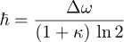
which is a Boltzmann distribution with β = ln2∕Δω. The identification ℏ = Δω∕ln2 connects the minimum frequency resolution of the spectral complexity measure to Planck’s constant. This is not a derivation but a precise identification that warrants further investigation.

3.2 Resolution of the Boltzmann Brain Problem

Under the Solomonoff prior P(s) ∝ 2^−L(s) applied to spectral complexity, the probability of a configuration is exponentially suppressed by its spectral cost. Chaotic, high-entropy configurations — Boltzmann brains, random fluctuations, disordered universes — have high spectral complexity: they require many high-frequency modes with large amplitudes to describe. Their probability under C_s is therefore exponentially suppressed relative to smooth, law-like, compressible configurations.

This resolves the Boltzmann brain problem without additional axioms. The selection of structured observers is not a fine-tuning accident. It is a direct consequence of the measure: smooth, predictable data compresses better than chaos, and the spectral complexity measure weights configurations by their compressibility. We do not find ourselves in a chaotic universe because chaotic universes are exponentially expensive to describe.