
Microscopic reality appears fundamentally wave-like. But as human observers, we do not inhabit an abstract, high-dimensional Hilbert space; we inhabit a tangible, three-dimensional geometry. Why? And more pressingly: why does matter cause this geometry to curve? Accepting the equations of General Relativity without understanding the deep, underlying reason for this curvature is one of the most profound frustrations in physics. We are told that mass bends space, but we are rarely told what space is actually made of such that it can be bent.
As Chapter From Nothing to Something demonstrated, a purely geometric interpretation of a random informational system starting from a state of zero entropy yields the curve
This curve grows rapidly at early times and flattens out as it approaches maximum saturation (Imax). We obtained this curve when starting from the all-zero bitstring and flipping bits randomly, one by one.
According to Chapter Humans as Axiomatic Systems, time is an internal property of observers, and that the universe must be fundamentally static, timeless and finite. It therefore has to operate on a strict, unyielding bit budget. What we observe as empty space must emerge from this static finite information — the execution trace of the computational equivalence.
We define the universe as n bits, giving a total of 2n possible configurations.
By sorting these configurations into increasing entropy order (the expanding entropy we observe) via random bit mutations, one obtains a typical thermodynamical system rushing toward full equilibrium (maximum entropy n).
Deriving Time. The only meaningful minimal time step in such a system is one bit-flip; randomly mutate bits, one by one, by randomly choosing either one or zero. Such a bit-flip space is natively logarithmic. From thermodynamics we know the system takes nlnn bit-flips to reach equilibrium and full saturation of entropy. Identifying one bit-flip with the minimum time resolution (a Planck time unit, tP ), the total time span is

The Space Size Function: x(n).
The number of bits also determine the maximum resolution for the spatial dimension of space.

Deriving the Aspect Ratio of Spacetime
By dividing spatial resolution with temporal resolution gives is something all graphics programmers are very familiar of - the aspect ratio. This time it is not a pixel aspect ratio of the monitor, but the aspect ratio of the nature.
During its first moments the evolution of the universe the size of the universe increased exponentially. This inflationary period corresponds remarkably well to an expanding thermodynamic system exploding from a zero entropy state.
During inflation, the universe expanded exponentially with speed measured using e-folds (N), where the size of the universe scales by a factor of eN.
According to the Standard cosmological models inflation lasted for about 10−35 seconds. During the period the universe expanded by at least 60 e-folds, meaning its size multiplied by a factor of e60, which is roughly 1026.
We can plug these numbers into our aspect ratio equation. But to get dimensionless aspect ratio we need to express both size of the spatial and temporal dimensions in the same units. According to physics there is minimal resolution for both distances and time, called Planck unit. So by expressing the size and duration of the inflatory period of the early universe in Planck units:


The dimensionless inflationary aspect ratio is then:

To solve the number of bits n corresponding thermodynamical system expanding with such a profile we set 𝒜(n) = 𝒜inf and solve:
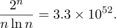
This equation has no closed-form solution and is solved numerically. Binary search over n ∈ [1,300] yields:
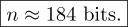
Verification: 2184∕(184 × ln184) ≈ 3.3 × 1052. ✓
We now know the number of the universe: it is: LARGE1052
Programmers are more familiar with binary systems. Mapping the above number to binary based gives us 2184 bits.
Modern computers are all 64 bit systems these day. 184 feels astonishingly small.
The total number of bits in the universe: ≈ 647.25 bits
We can apply this same equation to any event horizon, such as a solar mass black hole, to get the number of bits in it. By doing it we discover that we don’t get the exact same number as Berkenstein and Hawking through their black hole entropy laws. Our figure is off by 4π.
The reason for this is that the geometry of aspect-ratio we worked out is the aspect ratio of a rectangle. Based on all observable evidence, and even General Relativity, we don’t live in flat plane with open edges, more than we live on earth that is flat, as argued by flat eathers. According to GR’s we are living in an universe that must meet sperical symmetry. To turn surface area of a rectangle to sphere we must multiply by 4π, which gives us exactly the number Berkenstein and Hawking computed.
As an example, the size of the minimal Schwarzschild black hole radius the bit count would be ≈ 127 bits. Again, the difference to the bit count of the the entire universe ≈ 184 feels quite small.
In thermodynamics, a system with n bits starting at zero entropy (S = 0) maximizes its entropy when it has explored the configuration space uniformly.
With 2184 possible arrangements, a simple random walk of length nln(n) means the universe is still in the absolute infancy of its journey toward full equilibrium. The ”rush” toward heat death is barely even a single step into an unimaginably vast maze of states.
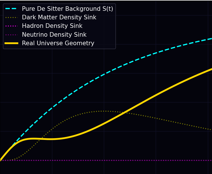
Einstein’s de Sitter Vacuum Solution describes exponentially and infinitely expanding empty space. When we map linear coordinate time to the logarithmic bit-flip time of our model, the linear expansion transforms into our statistical entropy curve. According to general relativity, empty space behaves as purely thermodynamical system rushing towards full saturation of entropy.
This naturally maps the event horizon (which expands at the speed of light in the Einstein manifold) onto a finite horizon of size 2n.
However, the universe is not empty space. It consists of matter and energy in form of particles. We observe electrons, positrons, quards, so called Hadrons making up matter. Energy takes the form of Bosons - photons, gluons, Higgs, to name a few. When these are injected into Einstein’s Stress Energy Tensor, the pure exponentially expanding De Sitter space turns into the currently observed reasonably expanding universe.
In the cosmic timeline, the pure, unblemished inflatory expansion only lasted for the opening act. At later times, neutrons, hadrons, and complex matter structures frozen out of the vacuum, deviating the cosmos from simple uniform entropic expansion.
If De Sitter is one extreme, then what is the other? It is called a black hole. It represents the other extreme end of General Relativity.
This naturally maps to another event horizon - the event horizon of a black hole. According to Berkenstein-Hawking the surface area of a black hole is proportional to its entropy. And entropy is a measure of information - a finite horizon of size 2n.
Are we on the right track? Let’s double check.
According to Berkenstein-Hawking theorems, the surface area of a black hole is proportional to its entropy. And entropy is a measure of information - bits.
So we can use the aspect-ratio hypothesis derived above to bypass Bekenstein-Hawking’s area formula entirely and derive the physical surface area of a black hole using the aspect ratio equation.
If a black hole is a localized thermodynamic system with n bits, its physical dimensions must satisfy the ”aspect ratio” rule.
The structural geometry equation for the black hole is:

The Bekenstein-Hawking calculates that a solar-mass black hole has an entropy of roughly 1077 bits.
If we plug this into our formula:

One Planck area is lp2 ≈ 2.61 × 10−70 m2.

A surface area of 3.76 × 10⁷ m2 corresponds to a sphere with a radius of about 1.73 km.
In standard astrophysics, a solar-mass black hole has a Schwarzschild radius of about **3 kilometers** (giving a surface area of roughly 1.1 × 10⁸ m2).
Our formula gets us to the exact same order of magnitude (107 to 108 square meters) entirely from a pure, information-theoretic ratio!
It adds up;  geometry correctly scales the massive information of a black hole down to its
tight, physical boundary without needing to plug in General Relativity constants like G or
c.
geometry correctly scales the massive information of a black hole down to its
tight, physical boundary without needing to plug in General Relativity constants like G or
c.
We have built a purely digital structural model for a event horizon.
We are not external observers. To understand curvature we must anchor the observer inside the system, constructed from the very same fluctuating informational currency she is trying to measure. In such a universe, distances cannot be gauged with an absolute external metric. Measuring rods must be built from the emergent structures of the universe itself.
From the outside, the universe would look like a simple informational gas expanding toward maximum entropy and flattening into a featureless state — a parabolic saturation curve. But we live inside. Our rulers are made of quarks, hadrons, and molecular bonds.
As global entropy increases, emergent structures precipitate out of the vacuum according to nested log-normal probability distributions. These structures are not added from outside; they are paid for from the fixed informational bit budget of the spacetime fabric itself.
Imagine an initial pristine patch of vacuum consisting of exactly 100 space-fabric tokens. When the first neutron freezes into existence and requires the informational equivalent of ten tokens, those bits are withdrawn from the active vacuum. The local spatial resolution instantly drops from 100 to 91. The same relational horizon must now be spanned by fewer tokens, stretching the background fabric. From the internal observer’s perspective — whose measuring rod has itself been redefined — space appears to have contracted locally.
As established in Paper III, the probability of emergence of structures in the increasing-entropy walk follows a log-normal distribution. This naturally explains the observed evolution in the ΛCDM model.
The early universe underwent a huge inflationary phase. Shortly afterward, photons, neutrinos, hadrons, quarks, and electrons emerged. The presence of matter slows the expansion (as described by GR), leading to the observed Hubble history. The baffling acceleration curve is explained by the log-normal probability density of emergent structures.
When the log-normal distribution peaks, the creation of complex matter structures peaks. Because these structures consume tokens from the finite entropic budget, the geometry we observe is the relational reflection of this balance. Early on, the rapid conversion of vacuum tokens into matter puts a statistical brake on perceived expansion. Later, as the log-normal tail decays, complex structures gradually dissolve, releasing tokens back into the vacuum. The local metric loosens. To an internal observer with a shrinking matter-based ruler, space appears to accelerate outward.
This framework also reinterprets cosmic heat death informationally: in the deep future, as the log-normal tails flatten toward zero, the probability of stable matter fades. All borrowed bits return to the background pool. The universe dissolves its structures and returns to pure, unblemished, static spacetime fabric — a simple, beautifully predictable statistical random system.
Let us recall our hourglass metaphor. There exists an astronomical, near-infinite number of ways to microscopically arrange individual grains of sand inside the lower chamber of an hourglass. Yet, despite this massive underlying microstate entropy, every single one of those chaotic configurations yields the predictable macroscopic geometric structure: a simple, uniform cone shaped stack of grains.
The physics of the hourglass acts as a spatial compressor - it compresses billions of independent, messy degrees of freedom into a geometric shape uniquely described by just a couple of macroscopic variables.
With sufficiently many grains, a small set of macroscopic constraints naturally generates simple large-scale geometries such as spherical planets.
To scale this logic to its absolute limit: given a 3 + 1 dimensional spacetime manifold, what is the highest possible compression efficiency a physical system could ever theoretically achieve?
The answer is a black hole.
The physics of black hole entropy represents the ultimate geometric data compression routine. One can throw any arbitrary arrangement of matter, information, or complex structures into an event horizon—guitars, spaceships, or burning stars—and the geometry instantly strips away their uncompressed, high-entropy descriptive overhead. What remains is a perfectly smooth, featureless region of spacetime governed by the No-Hair Theorem, fully specified by exactly three macroscopic attributes: mass (M), electric charge (Q), and angular momentum (J).
If the quantum mechanical wavefunction acts as nature’s spectral compression system, then what purpose does general relativity serve?
The answer is geometric compression. Even at the largest cosmological scales, what we are observing are compressed structures.
Under an information-theoretic framework, the both theories appear to be compression algorithms optimized for different informational domains, unified by a single imperative: the minimization of description length.
Dispite their differences, when evaluated through the lens of compression, Quantum Mechanics and General Relativity reveal many structural symmetries that standard physics treats as mere mathematical coincidences.
In Quantum Mechanics, observables emerge from operators acting on a Hilbert space. In General Relativity, gravitational structure emerges from invariant relations encoded in spacetime geometry. In both domains, stable physical content is defined by structures that survive changes of representation.
Neither theory stores absolute, localized information. Quantum Mechanics explicitly encodes the mathematical relations between measurement outcomes via complex probability amplitudes. General Relativity explicitly encodes the topological relations between events via the metric tensor of a spacetime manifold. In both systems, absolute, privileged reference frames are utterly discarded and replaced by pure relational networks.
Both architectures are strongly governed by global constraints. Unitarity in Quantum Mechanics preserves the conservation of total probability over time. In General Relativity, the Bianchi identities and the Einstein field equations tightly constrain how curvature can dynamically evolve.
Why should we find ourselves compressed by two separate systems? In terms of description length, utilizing two entirely different compression algorithms incurs a higher informational overhead. Why would nature implement two separate systems when one should suffice? Furthermore, why did nature favor the geometric framework of general relativity over the spectral domain of Hilbert space for our macroscopic reality?
As conscious agents, we are fundamentally finite informational structures. We cannot exist as diffuse, fluid, overlapping gradients. Observers require stable subsystem boundaries that preserve their information across time. Based on real world experience we know that happens if two highly complex, entangled informational systems were to spatially overlap and mingle their states even a little. Their internal data organization would instantly disrupt, causing immediate decoherence and a catastrophic loss of structural identity. Just dip your little toe into an acid - the consequences are catastropic.
To maintain informaitonal boundaries within a high-dimensional, fully entangled Hilbert space is computationally devastating, requiring an unsustainable expenditure of information.
However, boundaries can be defined very economically within a low-dimensional geometric space. Geometry grants us the gift of locality. It establishes the rigid, clear distinction between inside and outside.
The long-sought unification of physics is not achieved by violently forcing the linear mathematics of Quantum Mechanics into the non-linear tensors of General Relativity. Instead, it is achieved through Compressibility.
A purely spectral representation provides no native notion of localized boundary, inside versus outside, or persistent subsystem separation. Observers require such structures.
We inhabit geometric spacetime because geometry offers exceptionally low description length for defining informational boundaries.